Introduction to Atomic Trapping
What is Atomic Physics?
The taxonomy of scientific disciplines is often arcane and unintuitive, and physics is no exception. When one hears the phrase ‘atomic physics’, they might be tempted to assume some relationship to ‘nuclear physics’ – after all, what is an atom but a nucleus with bound electrons? Yet these two fields could hardly be more distinct, having entirely separate histories, techniques, and applications.
The theory of atomic physics typically considers individual atoms in isolation. In the early 20th century, this posed a seemingly insurmountable practical challenge – by what methods could one experimentally isolate an atom, so that those theories could be verified and further developed? At standard temperature and pressure, even relatively heavy atoms in gaseous form, such as xenon, travel at over 200 meters per second, rendering existing observational tools at the time useless for studying them. It was not until the late 1980s (more than 30 years after the development of the atomic bomb, a major breakthrough of nuclear science!), when Bell Labs scientists William Phillips, Claude Cohen-Tannoudji, David Pritchard, and Steven Chu (among others) designed and fabricated the first apparatus for slowing and controlling ensembles of atoms in a gaseous or vapor form – the magneto-optical trap. This signaled a turning point in the study of atoms; for the first time, scientists could now create gases of atoms slow enough to be studied by conventional (e.g. spectroscopic) methods.
This practically instantly opened the door for a new generation of atomic physics. For example, in that same year, Steven Chu went on to utilize optical tweezers, a particle-trapping technique that had hitherto only been utilized for controlling macroscopic particles, to isolate individual atoms from within a magneto-optical trap. It only took a few more years for several more incredible achievements in the field; for instance, in 1985, Eric Cornell and Carl Weiman were able to cool an ensemble of Rubidium-87 atoms to below 170 nanokelvin, creating the first ‘pure’ Bose-Einstein condensate, a state of matter in which all constituent particles are occupying the same state.
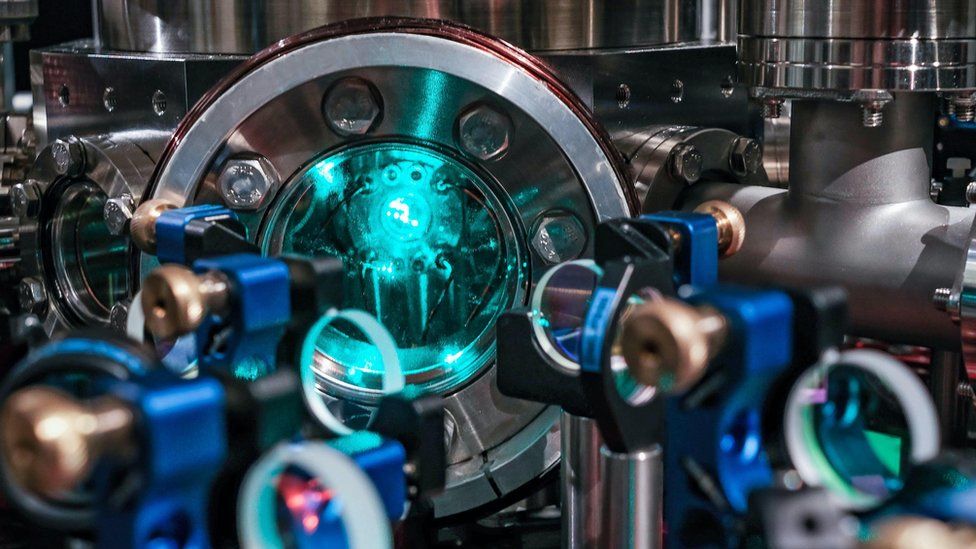
Nowadays, the magneto-optical trap (henceforth ‘MOT’) is ubiquitous in atomic physics labs, as it allows for researchers to experiment on individual (or arrays of individual) atoms. The objective of such experiments are typically investigating light-matter interactions, or how the trapped atoms behave under the influence of external electromagnetic waves. Modern uses of the MOT include quantum computation, atomic clocks (which have been proven to be the most precise timekeepers currently existing), and various quantum sensors capable of detecting even the most minute changes in signals. The field of atomic physics is so nascent that every year, several novel applications are published, making it one of the most exciting and fastest-growing branches of science.
Magneto-Optical Trapping
How does a magneto-optical trap work? The keys, as the name suggests, are coherent light (most commonly found in the form of lasers) and a sufficiently strong magnetic field gradient.
Magnetics
Since (non-ionized) atoms are inherently ‘neutral’ (having just as many electrons as protons), one might expect them to not interact with an external magnetic field. However, this is not the case – since the electrons and protons share a different spatial density (i.e. are not directly on top of each other), every atom will have a (typically very small) magnetic dipole moment. This allows them to interact, albeit weakly, with an applied magnetic field.
A magnetic trap works by creating an energy minima in a region of space through the interaction of the magnetic dipole with the external magnetic field. The spatial energy shift is given by:
\[\Delta E(\vec{r}) =- \vec{\mu} \cdot \vec{B}(\vec{r})\]where \(\vec{\mu}\) is the magnetic dipole moment and \(\vec{B}\) is the magnetic field vector. This creates a potential energy well, in which an atom, after equilibrating, would be found at the trough. However, analogously to classical mechanics, a ball rolling in a well may ‘escape’ that well if its kinetic energy is higher than the potential energy difference between the trough and peak of the valley. And, as mentioned earlier, atoms in gaseous or vapor form at room temperature and pressure move extremely fast – between this fact, and the relatively small magnetic dipole moment of neutral atoms, it would take an impractically strong magnetic field to trap room-temperature neutral atoms.
However, if the kinetic energy of the atoms were to be reduced, then at some point, we could use a reasonably large magnetic field to create a shift in energy sufficient enough to trap said atoms in a desired region of space. This is where the other half of the MOT comes in – the optics.
Optics
Electron Excitation
As Einstein theorized in the early 20th century, light is quantized, i.e. light waves are made up of individual particles known as photons. Atoms interact with light through their bound electrons, in a process during which an electron may absorb a photon and gain that photon’s energy. This process is known as electron excitation, and has a reciprocal process known as electron decay, in which an ‘excited’ electron may re-emit the photon it absorbed, and lose that photon’s energy.
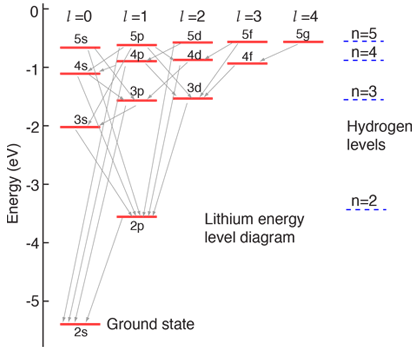
These levels, at first glance, appear to be separated by fixed, definite amounts of energy, and therefore one might expect that a photon must have some exact energy for the atom to absorb it. However, due to time-energy uncertainty, this is actually not the case; there is an ‘uncertainty’ inherent in the energy of the excited electronic state, which we denote the line width of the atomic transition. Moreover, by the time-energy uncertainty relation, the wider this line width is, the shorter the lifetime of the excited state (before it decays back to the original state), and vice versa.
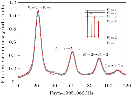
The line width of an atomic transition tells us what range of frequencies / wavelengths our laser has to be within to be able to excite the electrons in the atoms we’re shining it on. For an atom such as Rubidium-87, and a typical transition we might be interested in, such as the \(5^2 S_{1/2} \to 5^2 P_{3/2}\) (a ground state to a ‘first’ excited state) transition, this line width would be around ~38 MHz, which corresponds to a range of tens of femtometers in terms of wavelength. In other words, if we want to shine a laser on a Rubidium-87 atom such that it will absorb photons and undergo this transition, we need to make sure that our laser has a wavelength no more than about 40 femtometers from the central transition wavelength of 780,241,209 femtometers. The construction of such a laser is one of the biggest challenges in creating an atomic trap.
Doppler Cooling
Let’s assume we have a tunable laser with a sufficiently narrow bandwidth. How is it possible that we can make something colder using a laser? After all, if we are imparting energy to an ensemble of atoms, that should only raise the total kinetic energy of the gas.
The answer arises from the interaction between electronic excitation and the relativistic Doppler effect. You may be familiar with the aural Doppler effect, in which sounds being emitted by an object moving towards you are heard at a higher pitch, and then drop to a lower pitch as the object moves away from you. In short, the effect here is a shift of the wave to a higher frequency when it is approaching you; this occurs for light in a very similar way to sound.

In an atomic trap, an atom that is moving towards a photon from our laser will ‘see’ the photon as having a higher frequency (and therefore, energy) as we see it in the laboratory frame. Therefore, if we tune our laser so that its frequency is slightly below the resonant frequency, the only atoms that will be excited by our laser are the ones that are moving towards it, due to this Doppler effect.
These excited atoms will eventually decay back down to their ground state. When they do so, they can re-emit the photon they absorbed in any random direction. If they emit the photon in the exact same direction as it was traveling when it was absorbed, then by conservation of momentum, there will be no net change in the velocity of the atom. However, if it emits the photon in any other direction, there will be a net slowing effect on that atom (again, due to conservation of momentum).
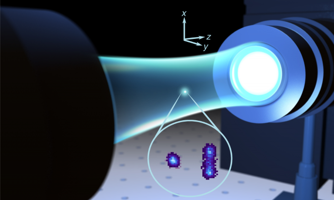
If you have three pairs of counter-propagating beams (ideally in pairwise orthogonal directions), then the net effect is to ‘push’ all the atoms towards the intersection point of these beams, which creates a ‘trapping zone’ for the atoms. When the magnetic trap, described above, is coincident with this beam overlap zone, we have successfully created a magneto-optical trap!
This is a simplified explanation of the workings of the apparatus; the exact mechanics are a bit more complicated, and require an understanding of quantum mechanics and the Zeeman effect. See Harold Metcalf’s Laser Cooling and Trapping for a complete reference.
Theory to Practice
The basic theory of a MOT is not overly complex; a student with a decent background in quantum mechanics might go through the derivations in a couple of weeks. However, such theoretical analyses often implicitly make assumptions about experimental parameters and ambient sources of noise, which in practice do not hold without careful design and assembly. Moreover, the majority of implementation-focused literature published on the subject of MOTs tends to focus on a specific aspect of the apparatus and omit the details relevant to the remaining components.
Thus, to fully understand the technical details and requirements for fabricating a MOT, one must study several papers and texts on each of the various sub-systems involved and then figure out how to assemble them, which can be a confusing and painful process. This work aims to provide a ground-up overview of the necessary components of a MOT for rubidium, implementation details on typical forms for each of those components (with a particular focus on minimizing cost), and a discussion of the motivation behind such implementation details.
The remainder of this project is organized into four sections. The first is a discussion of the source of light used to stimulate the canonical ‘cooling’ atomic transition of rubidium-87, including how to fabricate such a source, how to power and control it, the requirements that must be met, and the fundamental reasons for such requirements. The second is a discussion of the required ambient conditions for a MOT, how they can be achieved, and the motivations for such requirements. The third section is a discussion of the optical system that enables magneto-optical trapping, and how to design and implement such a system. The fourth and final section is an analysis the data collected during experimentation with my own personal build.